On Transparent Metagenomics

A Note on Terminology #

The terminology used to describe microbial communities is diverse and often subject to debate. Common proposed definitions are:

Microbiota

The assemblage of living microorganisms (bacteria, archaea, fungi, and viruses) present in a defined environment.

Metagenome

Strictly, the collection of genes and genomes from the members of a microbiota.

Microbiome

The entire ecosystem, encompassing the microbiota, their genomes, and the surrounding environmental conditions.

While these biological distinctions are important, in the literature (and within this post) the terms microbiome data and metagenomic data are frequently used interchangeably to refer to the high-throughput sequencing read count tables derived from these communities, regardless of whether the underlying biological material was the organisms themselves or their extracted genetic material.

Introduction #

In an ideal world, every research project would be perfectly reproducible. That is, anyone should be able to take the detailed description of your methods and reproduce your results, either with your data or with their own data. Much has been written about reproducible research, and in fact the field of metascience itself is primarily concerned with reproducibility. The concepts that I will describe here are not new. However, while the general ideas behind reproducible research are broadly the same in every field, transparent and reproducible reporting in metagenomics requires substantially more effort.

In metascience, a distinction between reproducibility and replicability is often made. Reproducibility is whether other scientists (including future you) are able to reproduce your analysis as-is, with your given data and code. Reproducibility, therefore, is primarily a matter of good housekeeping. Replicability, on the other hand, is more of a scientific concern. Are others able to find results that match yours in study populations other than the original study population? Both reproducibility and replicability are important, but we’ll start with reproducibility given that without reproducibility your results cannot be replicable. Reproducibility is necessary but not sufficient for replicability.

On Sampling Metagenomic Data #

While the majority of this post will deal with analysing and reporting on metagenomic data, it is important to recognise that metagenomic data is extracted from real biological samples. The physical act of sampling is inherently messy, and often the stage at which decisions can most drastically alter study conclusions. The journey to reproducible research begins the moment you collect that sample, long before the data ever gets to a computer.

Consider the simple impact of storage on two samples from the same individual. If sample x remains at room temperature on a lab benchtop for two hours while sample y is immediately stored in a −80°C freezer, you may generate drastically different microbial compositions. Differential degradation rates, sample lysis, as well as a host of other factors can impact extraction and replication efficiency. No downstream bioinformatics pipeline, regardless of how sophisticated, can magically recover information that is lost prior to sequencing.

Bit-rot and the End of Things #

Before I get to suggestions for a transparent metagenomic analysis workflow I need to point out that reproducibility is only as good as your available documentation. If you have great documentation on your workflow but absolutely nobody can find it, then unfortunately your study cannot be reproduced. I have lost track of the number of times I have searched for detailed methods for a metagenomics manuscript only to be met with this:

Often the links to the supplementary data maintained by the journals themselves point to moved or unavailable resources. While this is not your fault as an author, it is ultimately your responsibility. Therefore, rule number one of transparent metagenomics is:

You must have a permanent link to your detailed methods documentation that is attached directly to the manuscript and always points to the current documentation for said analysis.

Ideally, this would be located in the same place that your final analysis scripts are located, and the link to both of those things is somewhat permanent. A good option for this is Zenodo. See Zenodo’s github documentation for information on how to do this. Zenodo will not only provide a Digital Object Identifier (DOI) that links directly to your chosen repository, but will archive the version of your repository at the time you choose to publish on Zenodo. The exact data and code you used to generate your findings will be permanently linked to a specific identifier that is not tied to account names (which may change) or proprietary software enterprises. GitHub is usually pretty good at tracking account name changes, but sometimes it can still lead to dead links. Now that we are in agreement about having permanent documentation, you may be asking what it is you should document.

Pipeline Pathways #

At a minimum, the exact code you used for your analysis should be documented. However, metagenomic analyses typically involve complex data cleaning and preparation before any actual analysis. The decisions made in the data processing pipeline can drastically alter your final results. Every single one of the steps in the pipeline below has the potential to alter the final results if different choices are made. Much like Gelman’s garden of forking paths, although in this instance it is more like a forest of forking paths.

To complicate matters further, metagenomic analyses often depend on externally maintained resources for many steps in the QC pipeline. For example, taxonomic classification often makes use of reference databases like silva or greengenes — for 16S rRNA sequencing. Thankfully, all of these resources are typically versioned, and therefore you merely need to document the specific version of the resource that you used.

For quality control and contaminant checking, it is not enough to just record the names and versions of software that you use. Ideally you should report both the code that you used to identify contaminants and the final list of contaminants so that readers of your work can determine for themselves if your approach and its results are reasonable.

Versions and the Beginning of Things #

Metagenomic software moves fast. Not only are there new software packages for metagenomic analysis almost weekly, but existing software updates constantly. The results obtained by a script written today might not be reproduced if someone — including yourself — re-runs the script in six months time. In fact, many R and python users can attest to the fact that code written today might not even work six months in the future, and a typical metagenomic analysis script will depend on a large number of external software packages. An example of a very simple metagenomic analysis script is shown below.

library("TreeSummarizedExperiment")
library("mia")
library("breakaway")
library("vegan")
library("maaslin3")
library("ANCOMBC")
library("radEmu")

# I've excluded non-metagenomic software for brevity, but each of those packages has its own defaults.

root = rprojroot::is_rstudio_project

tse_analysis = readRDS(root$find_file("data", "processed", "tse_analysis.rds"))

# This is a typical command call
output_ancom = ancombc2(
  data = tse_analysis,
  assay_name = "counts",
  fix_formula = "hiv_status + bmi + age + months_post_partum",
  p_adj_method = "holm",
  pseudo_sens = TRUE,
  group = "hiv_status",
  struc_zero = TRUE,
  neg_lb = TRUE,
  alpha = 0.05
)

All of the external libraries used above, as well as the function calls (like ancombc2()), have two things that make reproducibility hard: implicit versions and implicit defaults. The options shown in the ancombc2 are not all of the available options in ancombc2 and as such, any option that is not explicitly set will be set to the default value the function expects. See this vignette for all the options you can set in ancombc2. If the default values have changed since you last ran your script, then your results will unfortunately also change.

Which leads me to rule number two for transparent metagenomics:

Everything should have a version number attached.

Ideally one would document all of the default options of all of the software used, but for modern metagenomics analysis contexts, this is almost always not a reasonable nor productive use of time. I would like to keep this post as software agnostic as possible, and therefore won’t go into detailed description of all of the available software for recording software versions. However, there are a few standouts that I can recommended.

If you are working in R only, then the venerable renv — via the renv.lock file — will record the versions of all of the R packages you use and all of their dependencies. In this way, you can hand off an R project to someone else and they should, in theory, be able to download and install the exact versions of all of the packages you used^[1]. rix is a modern contender that aims to not only snapshot your R packages, but also all of the required system dependencies for your analysis. rix uses the nix package manager and sources under the hood, but attempts to simplify interacting with nix through rix. Finally, if you find yourself working in more than one language often, then you might find pixi to provide a more frictionless versioning environment that the previous two packages.

A minimal pixi.toml to specify the required versions of the dependencies for your project. pixi will use this file to generate a pixi.lock file that has the exact versions and locations of all of your dependencies. With the pixi.toml and pixi.lock files, any collaborator can just type pixi install to reproduce the entire environment.

[workspace]
authors = ["Luke Hannan <luke@lukehannan.com>"]
channels = ["conda-forge", "bioconda"]
name = "microbiome"
platforms = ["linux-64"]
version = "0.1.0"

[dependencies]
fastexcel = ">=0.19.0,<0.20"
polars = ">=1.40.1,<2"
r = ">=4.5,<4.6"
r-qiime2r = ">=0.99.20,<0.100"
bioconductor-treesummarizedexperiment = ">=2.18.0,<3"
bioconductor-decontam = ">=1.30.0,<2"

The tools described above are both useful and incredibly powerful, but all of the tools mentioned far are mainly designed to version one part of the full lifecycle of a metagenomic analysis. Often, bioinformatics processing happens separately to data exploration and analysis and as such are versioned separately. Domain specific languages aim to address that challenge by allowing you to specify the entire data preparation and analysis pipeline in a DSL. Snakemake and Nextflow are the two most popular workflow managers in bioinformatics. The example below shows how snakemake allows you to reproduce the entire pipeline figure in a single easily versioned text file. Importantly, snakemake describes every step of your analysis and the causal pathways between inputs and outputs. We’ll come back to causal pathways and Directed Acyclic Graphs in the reproducibility section. It is able to figure out that in order to use data/dehost/{sample}_R1.fastq.gz as an input target for the taxonomic_profiling rule, the remove_host rule (and all of its upstream rules) must first be executed before taxonomic_profiling can be executed.

SAMPLES = ["sample_A", "sample_B"]

rule all:
    input:
        expand("results/taxonomy/{sample}_report.tsv", sample=SAMPLES),
        expand("results/functional/{sample}_genefamilies.tsv", sample=SAMPLES)

rule quality_control:
    input:
        r1 = "data/raw/{sample}_R1.fastq.gz",
        r2 = "data/raw/{sample}_R2.fastq.gz"
    output:
        r1 = "data/qc/{sample}_R1.fastq.gz",
        r2 = "data/qc/{sample}_R2.fastq.gz",
        report = "results/qc/{sample}.json"
    shell:
        "fastp --in1 {input.r1} --in2 {input.r2} "
        "--out1 {output.r1} --out2 {output.r2} "
        "--json {output.report}"

rule remove_host:
    input:
        r1 = "data/qc/{sample}_R1.fastq.gz",
        r2 = "data/qc/{sample}_R2.fastq.gz"
    output:
        r1 = "data/dehost/{sample}_R1.fastq.gz",
        r2 = "data/dehost/{sample}_R2.fastq.gz"
    params:
        index = "resources/GRCh38"
    shell:
        "bowtie2 -x {params.index} "
        "-1 {input.r1} -2 {input.r2} "
        "--un-conc-gz data/dehost/{wildcards.sample}_R%.fastq.gz "
        "> /dev/null 2>&1"

rule taxonomic_profiling:
    input:
        r1 = "data/dehost/{sample}_R1.fastq.gz",
        r2 = "data/dehost/{sample}_R2.fastq.gz"
    output:
        report = "results/taxonomy/{sample}_report.tsv"
    params:
        db = "resources/kraken2_db"
    shell:
        "kraken2 --db {params.db} "
        "--paired {input.r1} {input.r2} "
        "--report {output.report}"

rule functional_annotation:
    input:
        r1 = "data/dehost/{sample}_R1.fastq.gz",
        r2 = "data/dehost/{sample}_R2.fastq.gz"
    output:
        genefamilies = "results/functional/{sample}_genefamilies.tsv"
    shell:
        "humann --input {input.r1} "
        "--output results/functional/"

Once you have reached the end of your analysis, and you are ready for publication, there are two more things that you need to version control. Your analysis code itself, and your data. Without version controlled analysis code and data, all of the fancy dependency tracking mentioned above will be useless because your project will not be reproducible.

Versioning of metagenomic data is as challenging, if not more so, than versioning analysis code given the common scale of metagenomic data. While it is a crucial aspect of reproducibility, it is beyond the scope of this post. For a thorough overview of the challenges and best practices, see The metagenomic data life-cycle: standards and best practices and the EMBL-EBI training on submitting metagenomic data to ENA.

Finally, you also need to upload your analysis code. Git and GitHub are the defacto standards for uploading and storing your code. And as mentioned earlier, integrates well with Zenodo. There are many, many tutorials on using Git and GitHub, but if the aim is to just archive the final analysis code, using GitHub is the simplest option. Just click the green upload button in the interface shown below, and give your file upload a meaningful comment and you are done. Once the analysis has been published, the GitHub code can be permanently archived as described above.

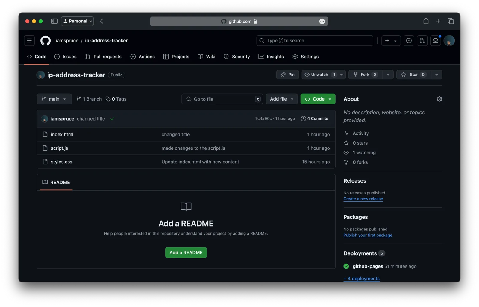
As a statistician or analyst, I believe advanced knowledge of git to be incredibly useful, both for version control and understanding the software you depend on, but for purely archival purposes directly interfacing with the GitHub web-ui will be enough for many researchers. Using the methods described above is sufficient to satisfy rule three of transparent metagenomics:

If it is mentioned in your manuscript, it must be online and accessible.

This excellent post by the Meren lab describes how paying lip service to data availability means nothing for reproducibility if interested parties cannot actually access the data. In particular, it shows that while the sequencing data itself is important, without the associated metadata it is functionally useless for answering epidemiological questions, and is at best fun training data for bioinformaticians.

Causes and Effects #

Reproducibility is necessary but not sufficient for replicability. Generating an exact in silico reproduction of an analysis is a good first step, but it cannot determine if the association you determined both exists in vivo and is causal. Therefore, in order to make sure your science is replicable there are two important considerations.

Firstly, are your results internally replicable. If you performed your analysis for a second time — from the beginning — using different but equivalent tools would you still come to the same conclusions. There are many alternatives for all the common tools used in metagenomic analyses. Often choosing between alternatives is a matter of preference not performance. Does choosing ANCOM-BC2 alter your final conclusions, compared to if you had used radEmu. If you re-run your k-means clustering algorithm with a different random seed do your results change entirely?

In metagenomic studies, the answer to both of the questions above is: likely yes. In fact, the analysis method you choose will drastically alter your final conclusions. Nearing et al. tested 14 different differential abundance algorithms across 38 datasets and found:

The percentage of significant ASVs identified by each DA method varied widely across datasets, with means ranging from 3.8–32.5% and 0.8–40.5%, respectively. Interestingly, we found that many tools behaved differently between datasets. Specifically, some tools identified the most features in one dataset while identifying only an intermediate number in other datasets.

Furthermore, both within and across tool differences in performance were altered depending on whether or not the datasets were filtered prior to analysis or not ^[2]. Unfortunately, it is not possible to accurately determine the true associations from false positive associations when the method you use is so sensitive to many possible differences in study design.

If your aim is differential abundance analyses, current recommended practice is then to run a variety of differential abundance methods and report concordance and discordance in the results generated by these tools. Reporting your results in this manner is much more work, but you gain much for your extra work. Reporting in this way allows you to explicitly report on the confidence of the associations you have found, and importantly when others are trying to reproduce your results they are able to discern which ASVs should reproduce and which might not due to the strength of the evidence.

This also allows you, the researcher, to be appropriately cautious in interpreting your findings: significant ASVs that do not reproduce across methods within your own study should be interpreted with caution. Particularly when working with sample sizes of typical metagenomic studies. The need for caution in interpretation is much greater when the aim is to evaluate the relationship between microbial relative abundance and health biomarkers ^[3]. This would lead to rule four for transparent metagenomics:

Make sure that your analyses reproduce within your study, across methods.

If you’ll indulge me one concluding footnote: in metagenomics, as in all science, the most important concerns of reproducibility are not technical — they are scientific. The recent article by Mitchell et al. illustrates many of the aspects discussed in this post. The title is: “Conceptual and methodological flaws undermine claims of a link between the gut microbiome and autism”. The fundamental issue it raises is not about software versions or dead hyperlinks; it is about whether the associations being reported are meaningful in the first place. In metagenomics, as in all observational science, association does not imply causation. Microbial relative abundances are compositional, Meaning every taxon’s apparent abundance is defined in relation to all others, a feature that makes standard statistical tests misleading without appropriate correction. and the associations we observe between community composition and health outcomes may reflect confounding, reverse causation, or simply artefacts of the garden of forking paths described above. Making genuine causal claims from metagenomic data requires either experimental intervention or very careful application of causal inference methods. Without that, a perfectly reproducible and internally replicable association study may still leave the most important scientific questions with unsatisfactory answers.

That question, the one that motivates almost all human microbiome research, is whether the microbiome can be modified to improve health. Probiotics, dietary interventions, and faecal microbiota transplantation are all downstream attempts to answer it in practice. But the intervention literature can only be as trustworthy as the observational literature that motivates it. If our reported associations are not reproducible, not replicable across methods, and do not reflect genuine causal relationships, then the clinical promise of the microbiome will remain perpetually just out of reach. Transparent, reproducible science is a prerequisite for doing research that is actually useful.

1. There are some caveats to this; see renv caveats. ↩

2. It will not come as a surprise to anyone that both filtering methods and their general utility are hotly debated topics in metagenomics. See Waste not, want not for a rough idea. ↩

3. Identifying reproducible biomarkers for microbiome association studies requires thousands of sample sizes. ↩